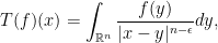
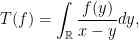
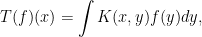
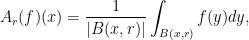
This week we come to the study of singular integral operators, that is operators of the form
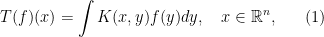
defined initially for `nice’ functions  . Here we typically want to include the case where
  has a singularity close to the diagonal

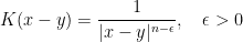
which is not locally integrable. Typical examples are
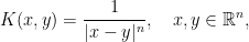

and in one dimension
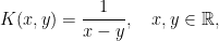
and so on. Observe that these kernels have a non integrable singularity both at infinity as well as on the diagonal  . It is however the local singularity close to the diagonal that is important and will lead us to characterize a kernel as a singular kernel. For example, the kernel
is not a singular kernel since its singularity is locally integrable. Observe that for Schwartz functions 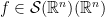 it makes perfect sense to define
and in fact the previous integral operator was already considered in the Hardy-Littlewood-Sobolev inequality of Exercise 12 in Notes 5 and can be treated via the standard tools we have seen so far.
Thus, if one insists on writing the representation formula (1) throughout  then will not be a function in general. Indeed, the discussion in Notes 4 reveals that if the operator
  is translation invariant then the kernel must necessarily be of the form
  for an appropriate tempered distribution
  :
:
Bearing in mind that there are tempered distributions which do not arise from functions or measures we see that (1) does not make sense in general and it should be understood in a different way. To give a more concrete example, think of the principal value distribution 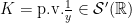 and write

Here we would like to rewrite this in the form
but this does not make sense even for  since the function
  is not locally integrable on the diagonal
  .
.
In fact, the representation (1) of the operator will not be true in general but we will satisfy ourselves with its validity for functions  , of compact support, and whenever
  does not lie in the support of
  . Indeed, if has compact support and
  then
then  in (1) and thus we are away from the diagonal. Indeed, returning to the principal value example, observe that the integral

makes perfect sense when has compact support and  . Continue reading →

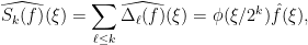
 be a smooth real radial function supported on the closed ball
  of the frequency plane, which is identically equal to
  on
on  . We then form the function
  as
as

 if
if  and also that
  if
if  we see that
  .
.
 forms a partition of unity:

 is supported on the annulus
  . Thus for each given
  there are only finite terms in the previous sum. In particular if
  , then

 . Some attention is needed concerning this point but usually it creates no real difficulty.
 and each
  is smooth and has frequency support on an annulus of the form
  . Now for
  let us define the multiplier operators
 . The operator frequency cut-off operator
  is almost a projection to the corresponding frequency annulus
 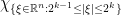 , introducing a small tail in the region
  which is mostly harmless. Similarly, the operator
  is almost a projection on the ball
  .
. 
 is of weak type
  and strong type
  . First of all we essentially used the fact that the linear operator
  and bounded, that is, that it is of strong type
  for every
  . Furthermore, the boundedness of the Hilbert transform on
  where
where  is the `good part’ in the Calderón-Zygmund decomposition of a function
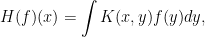
 and has compact support and
 boundedness of
  and then the corresponding boundedness for
  followed by the fact that
  around the point
  :
:
 is the Euclidean ball with center
  and
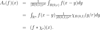
and  denotes its Lebesgue measure. Note that since Lebesgue measure is translation invariant we have
 denotes the Lebesgue measure (or volume in this case) of the
  -dimensional unit ball
  . Denoting by
  the indicator function of the normalized unit ball
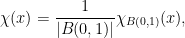
 and we define the Fourier transform in this set up. This will turn out to be extremely useful and flexible. The reason for this is the fact that Schwartz functions are much `nicer’ than functions that are just integrable. On the other hand, Schwartz functions are dense in all
  , so many statements established initially for Schwartz functions go through in the more general setup of
  such that the function itself together with all its derivatives decay faster than any polynomial at infinity. To make this more precise it is useful to introduce the seminorms
  defined for any non-negative integer
  as
as
 are multi-indices and as usual we write
  . Thus
  if and only if
  and
and  for
for  .
. and it is not hard to check that the more general Gaussian function
  , where
  is a
is a  , and each one of these spaces is a dense subspace of
  for any
  and also in
  , in the corresponding topologies.
 , the Fourier transform of
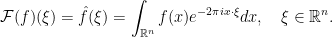
 denotes the inner product of
  and
and  :
:
 . It is easy to see that the integral above converges for every
  and that the Fourier transform of an
  . We have the following properties.
  and
and  for any
  .
.  is uniformly continuous.
 is bounded operator from
  to
to  and
and 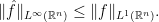
 . As we have seen the space
  to be the function

 is a Banach algebra.
 ,
,  , and
, and  , is a well defined element of